Exact Formula For Amount To Be Returned Is

P R T where P Principal R Rate of Interest in per annum and T Time usually calculated as the number of years. To calculate the annualized return we will be using the below formula.

Pin On Excel Functions

There are 3 levels therefor 3 tier payouts possible.

Exact formula for amount to be returned is. A1A2 returns TRUE To compare text strings in a case-sensitive way you can. F2 is the value which you want to return its relative information A2D12 is the data range you use the number 2 indicates the column number that your matched value is returned and the FALSE refers to the exact match. Both of the above formulas ignore non-text values such as errors booleans numbers and dates.

The formula to be used is SUMPRODUCTEXACTE3B3B8C3C8. Where The net return is the amount that a firm receives from its investments. Although there are several formulas to calculate ROI the two most common methods are listed below.

We have a different set of data as shown below. The above formula will run a test on the values in column B then convert the resulting TRUEFALSE values to 1s and 0s. IFA1B1 SUMA1D1 The formula compares the values in cells A1 and B1 and if A1 is not equal to B1 the formula returns the sum of values in cells A1D1 an empty string otherwise.

If Cell Contains Specific Text Then Return Value Using SEARCH Function. The only way for you to determine the exact refund amount for the IRS Where is My Refund tracker is to look at your tax return. In our example we have input data in Cell A2A12 and We will Return the Values in Range B2B12.

As stated this is only an estimation as a 6 rate would take 1190 years using the actual doubling time formula. The formula compares the values in cells A1 and B1 and if A1 is greater than B1 it multiplies the value in cell C3 by 10 by 5 otherwise. The INDEX function then returns the 7th value from the range C5C12 as a final result.

Too big Just combine it with your condition. INDEX C5C12MATCH F4 B5B120 INDEX C5C127 150. Highlight cells that equal.

Let understand the working of EXACT function in Excel by some EXACT Formula example. Value if false opposite to previous part this is a value returned if condition is false. The costs are those expenses that a business incurs during operation during.

For example a rate of 6 would be estimated by dividing 72 by 6 which would result in 12 years. How to Use EXACT Function in Excel. Below is the Excel formula to find If Cell Contains Specific Text Then Return Value.

The MATCH function locates the code ABX-075 and returns its position 7 directly to the INDEX function as the row number. The rule of 72 is found by dividing 72 by the rate of interest expressed as a whole number. First lets find the gain in investment which is the difference in Investment and final investment.

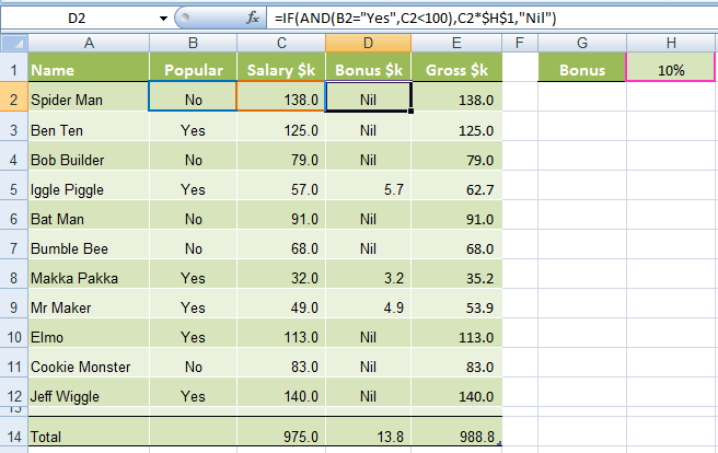
The first part of my formula is working and returning the correct dollar amount but the part that has 100 in. Then by dividing the amount of total return calculated above by the amount of investment made or opening value multiplied by 100 as the total return is always calculated in percentage. The reason we use a double negative is that it converts the resulting TRUE FALSE values to 1s and 0s.

The formula is solved like this. SUMIFA2A8C2C8 - includes seemingly empty cells that contain zero length strings returned by some other formulas eg. Maybe you will get the refund in your bank account before you.

BeginalignM 2xy - 9x2hspace025inM_y 2x N 2y x2 1hspace025inN_x 2xendalign So the differential equation is exact according to the test. For example with APPLE in A1 and apple in A2 the following formula will return TRUE. The First Method is ROI Net Return on Investment Benefits Cost of Investment 100.

In the above formula. First identify M and N and check that the differential equation is exact. Return value in another cell if a cell contains certain text IFISNUMBERSEARCH Yes D5 Approve No qualify Notes.

I am trying to get my formula to return a certain dollar amount based on the number entered and where it falls related to the goal. How to return a value instead of TRUEFALSE with IFORAND statement Just remove the OR. Following formula will return a A1 cell value if less than 5 and too big literally if A1 s value is bigger or equal to 5.

A loan amount is required to be returned by the person to the authorities on time with an extra amount which is usually the interest you pay on the loan. Total Return Formula is represented as below. The EXACT function in Excel is very simple and easy to use.

Unfortunately there is no one at TurboTax that can provide you with that number. Simple Interest Formula Simple interest is calculated with the following formula. Total Return Formula Closing Value Opening Value of Investments Earnings therefrom.

R Invest Amount GainInvest Amount 365Days-1. For example X1Y1 returns the same value as EXACTX1Y1. You can also achieve this by using Search Function.

Oobleck Setting The Scene 6 Space Probe Star System Scene

Inflation Adjusted Return Definition

Fv Function In Excel To Calculate Future Value Ablebits Com