
Using the example above you can get the value from the field Total in a record where color is red and Day is Tue with either of the two formulas below. This will ensure that A2 and D2 are first evaluated then divided by two.
Date Function Calculate Working Days With Networkdays Function In Ms Excel Excel Tutorials Excel Excel Formula
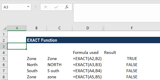
Exact formula in excel in hindi. TRUE Approximate Match और FALSE Exact Match. Get Certified Now Recommended. Using this rule we can rewrite the above formula as A2 D2 2.
Important points to keep in mind about HLOOKUP. You can download this Translate Excel Template here Translate Excel Template. Here I will take sum up for instance.
Professional financial modeling designation. Press F4 one time C2 will change to C2. I create a named formula.
A formula is a mathematical expression that you enter into a cell of your worksheet. A formula can also be used to calculate values such as profit margin or cost. Ad CFI Delivers an Outstanding Online Education for Any Aspiring Finance Professional.
DATE TIME SERIES FORMULAS. Ad CFI Delivers an Outstanding Online Education for Any Aspiring Finance Professional. The result would be 72.
Enter the value 1 for the first quartile. IMPORTANT TOOLS IN EXCEL. Here is how the F4 shortcut would work.
The INDIRECT function returns the value of A1 for use in formulas. Vlookup With Define Name 310 Start. Now go to B1.
You can take advantage of data validation to specify the type of data that should be accepted by a cell ie. Press F4 three times C2 will change to C2. DGET B7E14Total B4E5 field by name DGET B7E144 B4E5 field by index.
04654 HYPGEOMDISTA2A3A4A5FALSE Probability hypergeometric distribution function for sample and in cells A2 through A5. The formula used is TIMEVALUELEFTTEXTE2100002RIGHTTEXTE2100002 The outer function is the TIMEVALUE and it takes the text as time. Excel MAX IF formula Until recently Microsoft Excel did not have a built-in MAX IF function to get the maximum value based on conditions.
Pass the value 0 as the second argument to calculate the minimum value of the given data set. In any of your formulae you can check if xl_FR is truefalse and use jj or dd accordingly. ARITHMETIC OPERATORS SUM AVERAGE COUNT etc.
Now type CLEAN A1 excluding the quotes and then press Ctrl-Enter to apply the CLEAN function to the entire selection and clean every data point on our list. Vlookup with IFERRORFind Duplicate 334 Start. Select a blank cell you want to output the result and click Formulas Insert Function.
Although the latter 3 arguments of TREND are optional it is recommended to include all arguments to. Excel spreadsheet formulas usually work with numeric data. Enter the value 3 for the third quartile.
Fine Duplicate 156 Start. In the Insert Function dialog specify a function category in the Or select a category box and select a function from the Select a function list. Vlookup with IF and ISERRORFind Duplicate 259 Start.
CONCATENATE UPPER LOWER PROPER LEFT RIGHT TRIM EXACT etc. Hope this helps Hadi. FILTER SORT FREEZEREMOVE DUPLICATES CONDITIONAL FORMATTING.
It is a case. Where known_ys and known_xs refer to the x and y data in your data table new_xs is an array of data points you wish to predict the y-value for and const is a binary argument for calculating the y-intercept normally or forcing the value to 0 and adjusting the slope values so that. Using the SHIFT key select B1 to B1000.
EXPLANATION OF THE FORMULA. This is how I cope with their issue. Vlookup with Approx Match 154 Start.
We pick the left two digits with the help of LEFT FUNCTION and right two digits with the RIGHT FUNCTION. IFE7YesF5008250 In this example the formula in F7 is saying IFE7 Yes then calculate the Total Amount in F5 825 otherwise no Sales Tax is due so return 0. Follow the below steps to convert words into other languages.
Professional financial modeling designation. Now we will see the below option on the. You can easily create an Excel formula using this function and it.
Description Result HYPGEOMDISTA2A3A4A5TRUE Cumulative hypergeometric distribution function for sample and population in cells A2 through A5. Sorry to answer here for those using the french version of MS Excel. Xl_FR for ex Refers to.
Enter the value 2 for the second quartile. As we are looking out for an exact value it would be False. For example suppose you have the reference C2 in a cell.
It makes HLOOKUP search for exact or approximate value. CONVERSION OF MILITARY TIME TO STANDARD TIME. The next is range_lookup.
Here HLOOKUP is searching for a particular value in the table and returning an exact or approximate value. So the formula in E2 is saying IFActual is Greater than Budgeted then Subtract the Budgeted amount from the Actual amount otherwise return nothing. 13Vlookup with Absolute Reference in Hindi 504 Start.
Press F4 four times C2 will change back to C2. D d Click OK. Press F4 two times C2 will change to C2.
In the example hold Shift and click cell B1000 to select cells B1 through B1000. Vlookup Hlookup Syntax 529 Start. Pass the array or cell range of data values for which you need to calculate the QUARTILE function.
Go to the REVIEW tab and click on Translate. A while ago they introduced MAXIFS and now the users of Excel 2019 and Excel 2016 included with Office 365. Basic Vlookup 332 Start.
Get Certified Now Recommended.
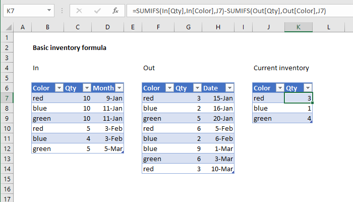
Excel Formula Basic Inventory Formula Example Exceljet
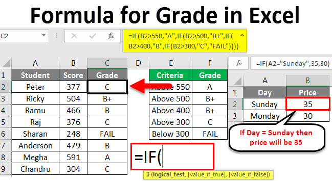
Formula For Grade In Excel How To Use Formula For Grade In Excel
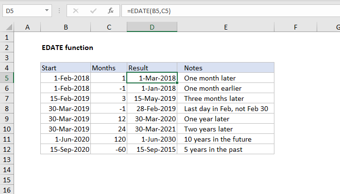
How To Use The Excel Edate Function Exceljet